Outside of art, I've also utilized some of my coding skills to create data analysis tools for scientific research. For this article, instead of walking through the code like a tutorial, I thought it might be better to just introduce some of the concepts that are utilized. That way, even if the specific project isn't relevant to you, the concepts might pique your interest.
This first article will go over the topics used in a tool I developed for this paper, with the purpose to analyze and quantify the ordering of particle assemblies. In simpler terms, given an input image of an ordered array of objects, this script outputs figures and numbers that describe how "well ordered" the assembly is. For an example, in the figure below the input image is an EM (electron microscopy) image of an array of polystyrene particles. The output image highlights areas of order, with a square pattern being shown in blue and a hexagonal pattern shown in red. These orderings are described as having 4-fold symmetry and 6-fold symmetry, respectively.
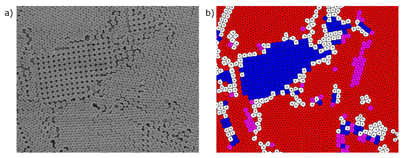
(a) A scanning electron microscopy (SEM) image of polystyrene particles. (b) A corresponding voronoi diagram colored according to symmetry. Blue indicates four-fold symmetry, red indicates six-fold symmetry, and purple cells meet the requirements for both.
By the way, the diameter of the particles imaged above is around 900 nm. For comparison, that's around 30 times smaller than that of a human skin cell!
In the script, two main steps occur. First, the input image is processing using image analysis techniques to identify particle center coordinates. Then, a bunch of math is performed to quantify ordering using those coordinates.
Image Analysis
Since you could take a whole course on image analysis, I'm only going to cover a few basic things. The first of which is image binarization. A binarized image is represented by an array of 1s and 0s, with each number representing a pixel. To get to this state from a colored image, you first convert to grayscale. Generally, in a grayscale image each pixel is represented by a value between 0 and 255. We can then choose a threshold value (say, 100), and convert all pixels above the threshold to 1, and all those below to 0. And just like that, we've successfully binarized our image. You can do other fancy things like adjust your threshold across your image based on local brightness to get a more accurate binarization. An example of binarization is shown below,
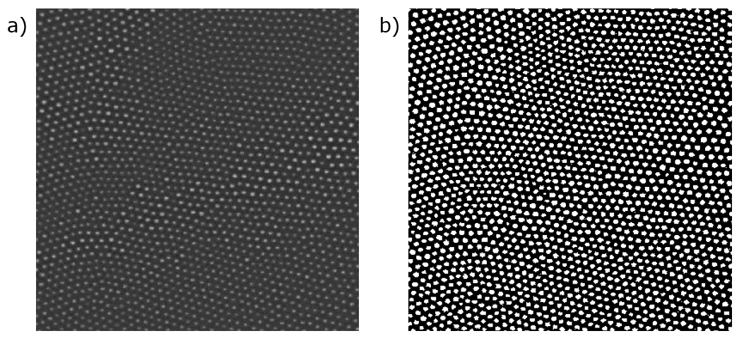
(a) A grayscale image of a particle assembly. (b) A binarized version of the image.
The next step is to clean up the binarized image, which is done using something called morphological operations. I won't explain in depth here, but they can be used to eliminate gaps or islands caused by noise. If you're interested, this page goes over the topic in more detail, and if you are really interested, this lecture provides a great overview. With the correct choice of operations, we can clean up our image as shown in the figure below,
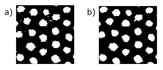
(a) A binarized image of a particle assembly. (b) The same image cleaned up using morphological operations.
Now that each object is isolated, we can individually pick out the region that defines each, as shown in (b) of the figure below. Then, we can find the center, or centroid, of each area by calculating the average of the pixel locations/coordinates that make up the area. The resulting centers are shown in (c) below,
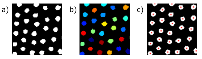
(a) A cleaned, binarized image of a particle assembly. (b) Segmentation of the image to identify individual particles. (c) Identification of particle centers.
With these coordinate centers, we can now perform some math to quantify their ordering.
Oh, and the steps above can only really be used when the objects have reasonable spacing between them. If the objects are closely packed together (like in the first figure of this article), we have to perform some extra steps. For the pros out there, I (1) perform a grayscale image opening with a disk, (2) binarize the image, (3) perform a distance transformation coupled with a Watershed transformation, and (4) mask the Watershed transform with the binarized image from (2).
Math Stuff
In order to perform most of the math, we need to identify each particle's neighbors. This may seem easy by eye, as obviously a particle's neighbors are those that are closest. However, the question comes down to how many neighbors a particle has. You could choose the closest four particles, or the closest six, or the closest twenty, etc. To perform this association quantitatively, we use a technique called a Delaunay triangulation. I won't go into detail on how this works, but you end up with something like the result shown in (b) below. The Delaunay triangulation can also be used to generate something called a Voronoi diagram, shown in (c). Within a Voronoi diagram, the cell around each point contains all of the area in which that point is the closest.
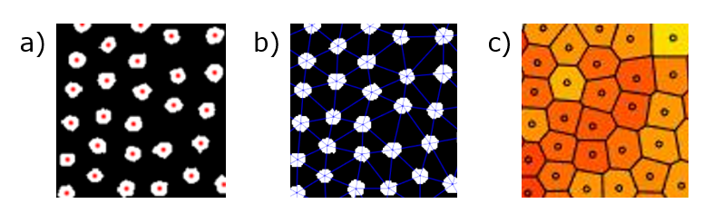
(a) Identified particle centers. (b) Delaunay triangulation of particle centers, connecting neighbors by a line. (c) Voronoi diagram of the particles. Neighbors share an edge.
Now that we have each point's neighbors, we can calculate a bunch of parameters including the number of neighbors and the distance to the nearest neighbor. One parameter I want to go over is called the local bond orientation order. It is calculated for a given point using the equation,
$$\Psi_s=\left|\frac{1}{N}\sum_{j=1}^N e^{i s \theta_j}\right|$$
Where s is either 4 for square packing or 6 for hexagonal packing, N is the number of neighbors, and θj is the angle between a reference axis and the line between the point of interest and neighbor j. i represents the imaginary unit. While I won't go into how this equation is calculated, I'll attempt to explain what it's calculating and how it works.
In simplest terms, Ψs represents how close a point is to having s-fold symmetry, varying from 0 to 1. For example, a point with perfect hexagonal symmetry with its neighbors would have a Ψ6 value of 1. The equation can be visualized as taking each neighboring point, and multiplying the angle between it and the reference axis by s. An animation of this is shown below, with the reference axis being the positive x-axis, shown in blue.
Visualization of the Ψ6 calculation for points with perfect hexagonal order. The angle between each point and the x-axis is multiplied by 6.
Since each point is 1/6th of a rotation away from each other, when rotated they end up all stacked on top of each other. The circle in red represents the average location of all the neighboring points. Once the rotation is complete, the distance of this red circle to the center is equal to Ψs. Thus, in the figure above, Ψ6 ends at its maximum value of 1. If we slightly offset the neighbors from perfect 6-fold order, we end up with Ψ6 values slightly below 1, such as in the figure below.
Visualization of the Ψ6 calculation for points with imperfect hexagonal order. Notice that the final Ψ6 value has decreased from 1.
If we then choose an arbitrary threshold for identifying a point as having s-fold order, say 0.8, we can now color code a Voronoi diagram of our input image to highlight regions of 4-fold and 6-fold order. In the figure below, blue represents points that have Ψ4 > 0.8, red for Ψ6 > 0.8, purple for both, and white for neither.
Now, you may be wondering what the φ value represents. This is called the "phase angle", and in our visualization represents the angle between the red circle and the reference axis. In the context of our input images, this represents the orientation of the hexagonal or square lattice. For example, if we offset our visualization by 𝜋/6, we end up with a φ value of 180° as opposed to the 360° (or 0°) we got before,
Visualization of the Ψ6 calculation for points with perfect hexagonal order with an offset of 𝜋/6. Notice that the final Ψ6 value remains at 1, but the final φ value is now 180°.
If we color our Voronoi diagram based on the φ value for each point, we end up with a really interesting (and pretty) result. Note this is a zoomed-out version of the figure shown earlier.
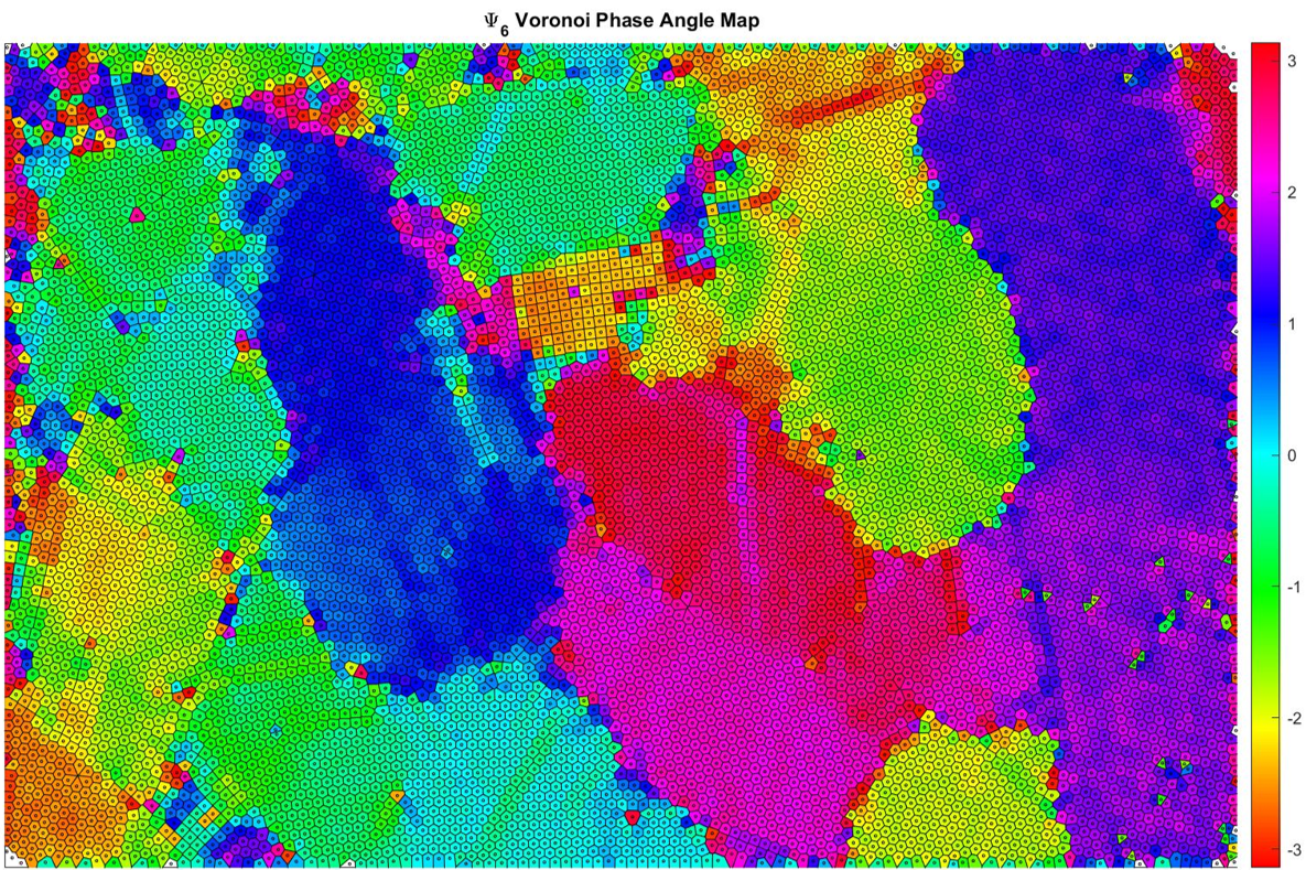
The voronoi diagram of an entire particle assembly. Cell color corresponds to the lattice orientation (φ) at that point.
If we compare this to the input image, we can see that each color corresponds to a region with a lattice in a distinct orientation,
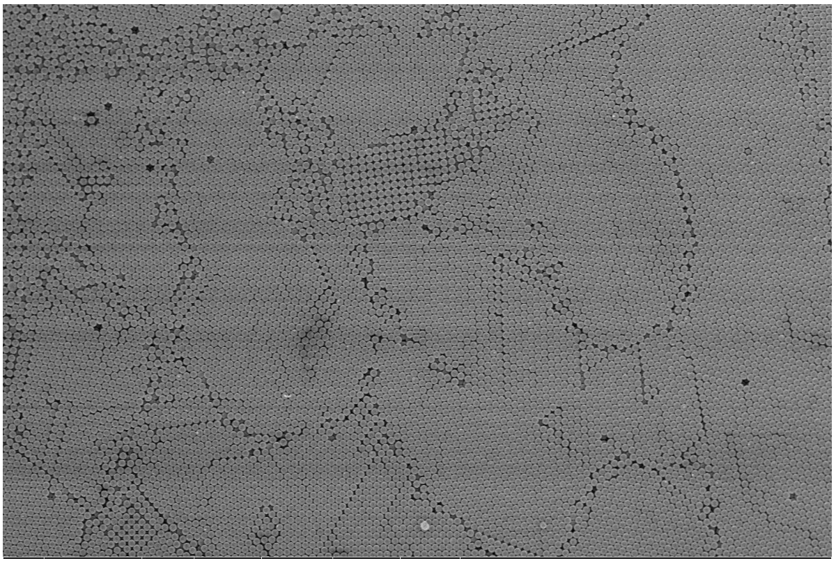
Scanning electron microscopy (SEM) image of a particle assembly. Input image for the voronoi phase angle map in the above figure.
Surprisingly, the rainbow coloring serves an additional purpose as opposed to just making the images look nicer. Since a φ value of 0° is only one degree apart from a value of 359°, this color scheme allows us to wrap between the two values, with red lying on both ends of the spectrum. Another interesting property to note is the relationship between φ and θ. For 6-fold order, φ ranges from 0° to 360° as θ ranges from 0° to 60°, since a hexagon rotated by 60° remains the same. Likewise for 4-fold order, φ ranges from 0° to 360° as θ ranges from 0° to 90°, since a square rotated by 90° remains the same.
Wrap Up
As usual, props to you if you made it through the whole thing. While this specific project is unlikely to be useful to you, I hope a few concepts stuck with you. Image analysis is a really powerful tool, and I've seen a few art pieces making really good use of Voronoi diagrams and Delaunay triangulations. Additionally, the Ψs equation and its visualization are very similar to that for the Fourier transform, which 3Blue1Brown has a great video on.
I'm not going to post the code for this one (mostly because it was written in MATLAB), but there are many libraries and scripts out there in pretty much any language for both image analysis and Voronoi/Delaunay calculations. If you're curious as to what this code is useful for, it was used in the journal article I mentioned earlier, where it was used to asses the long range positional and orientational order of particle assemblies. For many applications, particle ordering over large length scales is essential, and the values calculated using this script were used to prove that our assemblies could remain ordered at pretty much any size.